myCoolblue von Condair
Functional description and instructions
for the myCoolblue simulation software
The myCoolblue app is a powerful simulation tool that enables you to calculate the annual amount of energy required to cool and dehumidify the supply air to a ventilation system at a particular site. This means that you can estimate the expected energy-related benefits of employing indirect evaporative cooling in a ventilation system, based on actual climatological conditions, as early as the planning stage of a project. This in turn enables you to optimize the system’s components early on to ensure that it is as efficient as possible.
Fig. 1 Menu option - myCoolblue
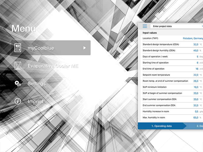
1 Menu option - myCoolblue
When you start the app, the menu appears. (see fig. 1.).
The myCoolblue option is selected automatically. Tap it to start the simulation
Fig. 1.1 Menu option — ME Evaporative Cooler
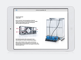
1.1 Menu option — ME Evaporative Cooler
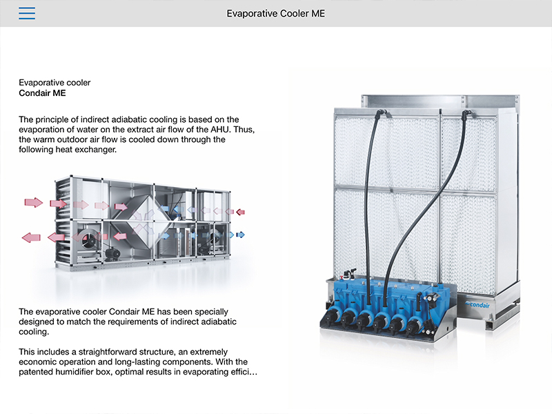
This section provides a brief overview of the technology and features of the Condair ME.
The Condair ME evaporative cooler is used as the basis for system-specific calculations carried out as part of the simulation. Performance data for other manufacturers may vary from this, so the simulation results apply only to those achievable with the Condair ME.
(see fig. 1.1).
Fig. 1.2 Menu option — Settings
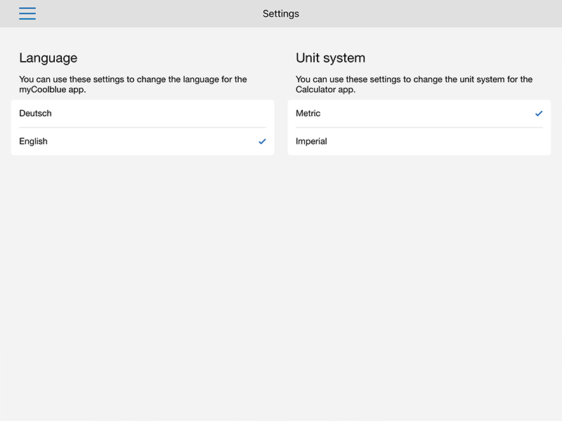
1.2 Menu option — Settings
Here you can set the language to either German or English, and select either metric or imperial measurements.(see fig.).
Fig. 1.3 Menu option — Imprint
1.3 Menu option — Imprint
Information about Condair GmbH as required under German law.(see fig.).
Fig. 2.1.1 Enter project data
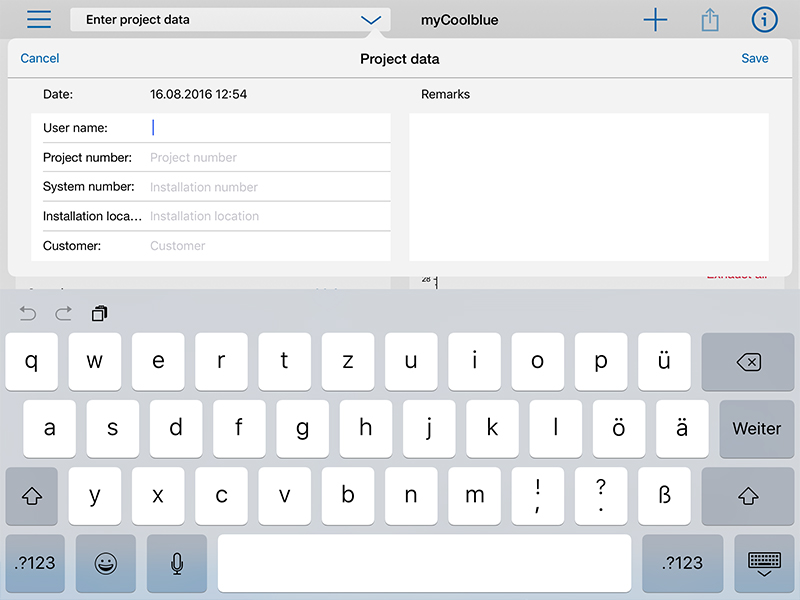
2.1.1 „Enter project data“
In this section, you can enter information about the simulation project such as the contact name, project name, location, system ID and customer name. You can also enter additional notes as needed. Tapping the Save button saves the data for use in the simulation. The information provided will also be printed on the datasheet (see fig. 2.1.1).
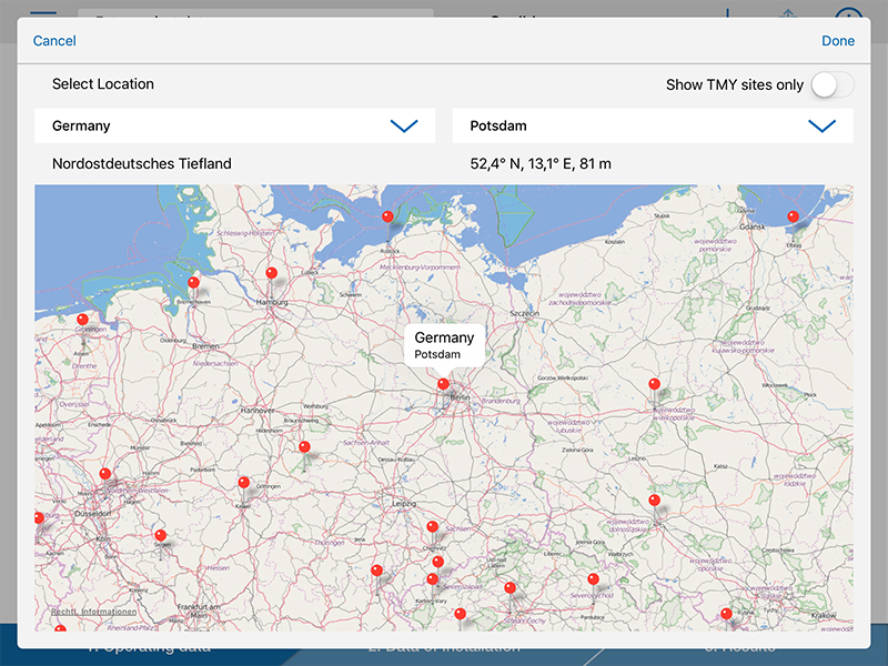
Fig. 2.1.2 Location selection
2.1.2 „Location selection“
The myCoolblue app includes 346 locations from around the world, some of which also serve as representative stations for their meteorological regions. The locations are marked on the world map with red pins, and can be selected with a simple tap.
Alternatively, you can select a location from a list by first selecting the country, then the specific location. Additional information is displayed for certain locations assigned to specific climate regions. The geographical coordinates for the selected location and its elevation above sea level are also displayed.
The calculations are based on current data from the new Typical Meteorological Years for average weather conditions (TMY) provided by Germany’s national meteorological service, the Deutscher Wetterdienst in Offenbach, and from Meteonorm 7.1.10. An additional filter allows you to select from TMY locations only (see fig. 2.1.2).
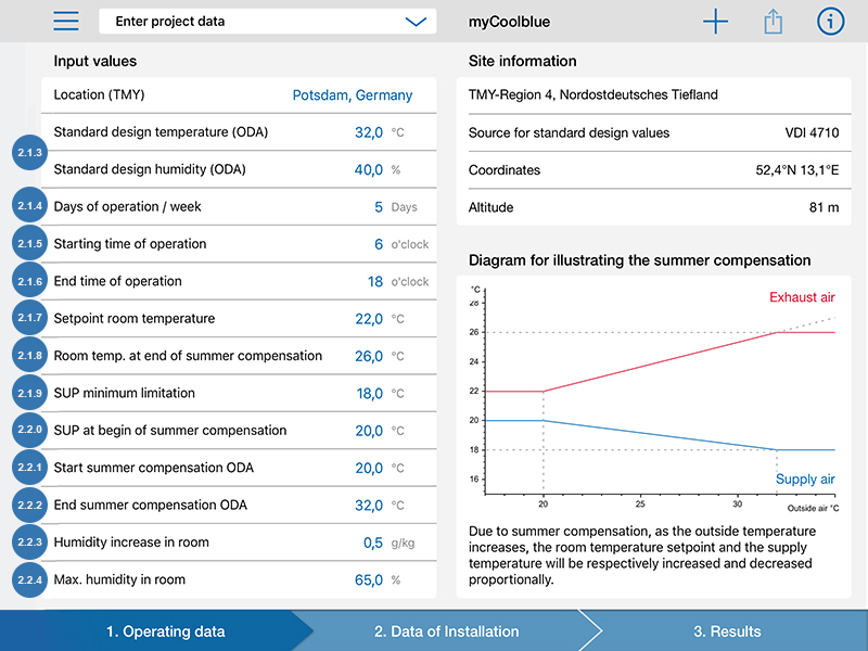
2.1.3 „Standard design temperatur/humidity (ODA)“
The design values for summertime temperature and enthalpy that are typically used to determine the dimensions of the chiller and the HVAC system at the selected location (see fig. 2.1.3).
In contrast to the operating point from the dynamic simulation, the capacity rating for the required chiller can be calculated based on a static design point. The required cooling capacity based on this design point will be included in the simulation results when the appropriate option is selected.
The temperature and enthalpy values shown for the selected location are based on design data from the Association of German Engineers’ standard VDI 4710, sheets 1, 3 and 4, and from Meteonorm’s meteorological datasets. The values provide for an annual frequency of exceedance risk of no more than 0.1%.
Note: ASHRAE (American Society of Heating, Refrigerating and Air Conditioning Engineers) sometimes provides different values for the frequency of exceedance risk, e.g. 0.4%, 1% or 2%.
.
2.1.4 „Days of operation / week“
Number of days per week the ventilation system will be operated (see fig. 2.1.3).
2.1.5 „Starting time of operation“
Time that the ventilation system will be switched on in 24 hour format. For example, if the system will be switched on at 7 in the morning, enter 7 here (see fig. 2.1.3).
2.1.6 „End time of operation“
Time that the ventilation system will be switched off in 24 hour format. For example, if the system will be switched on at 6 in the evening, enter 18 here (see fig. 2.1.3).
2.1.7 „Setpoint room temperature“
Desired temperature for the room or exhaust air. The room or exhaust air temperature will normally be governed by this value until summer compensation is activated. The default value is 22°C (see fig. 2.1.3).
2.1.8 „Room temperature at end of summer compensation“
Enter the room temperature you intend to have at the end of summer compensation. The default value is 26°C.
Summer compensation is used during the summer months to reduce the difference between the internal and external temperatures, thereby making entering or leaving a conditioned room a more pleasant experience. The target value is raised automatically and continuously, maintaining a defined difference between itself and the external temperature. Summer compensation also helps to save cooling energy by allowing room temperatures to be higher when it is warmer outside (see fig. 2.1.3).
2.1.9 „Supply air minimum limitation“
Enter the minimum supply air temperature at the end of summer compensation here. The temperature should not drop below this level. The default value is 18°C.
In a conditioned area, colder supply air is normally fed into the room to hold the temperature constant. This balances out the internal thermal load and the warmth brought in from outside. If the temperature outside is increasing, the amount of warmth entering from outside also rises. This can be compensated by simultaneously decreasing the supply air temperature.
(see fig. 2.1.3).
2.2.0 „Supply air at end of summer compensation“
Enter the supply air temperature which will normally be required to achieve the desired room temperature before summer compensation is switched on. The default value is 20°C (see fig. 2.1.3).
2.2.1 „Start summer compensation outdoor air“
External temperature at which the room temperature will start being raised or the supply air temperature will start being lowered. The default value is 20°C (see fig. 2.1.3).
2.2.2 „End summer compensation outdoor air“
Outdoor temperature below which the room temperature will no longer be raised and the supply air temperature will no longer be lowered. It is recommended that you use the value for the default outside air temperature here. The default value is 32°C (see fig. 2.1.3).
2.2.3 „Humidity increase in room“
Internal sources of humidity, such as people or technical processes, can have a negative impact on the exhaust air temperature that can be achieved through evaporative cooling. Any exchange of air with non-air-conditioned rooms or with outside air should also be taken into consideration, if present. To take this factor into account in the simulation, enter the internal moisture load here. If you do not have a precise figure, the default value is 0.5 g/kg (see fig. 2.1.3).
2.2.4 „Max. humidity in room“
The maximum value for room humidity also affects the exhaust air temperature achievable through evaporative cooling. A low value will reduce the energy share used by the evaporative cooling system over the course of the year due to the higher proportion of energy being required for dehumidification. The standard value is 65% (see fig. 2.1.3).
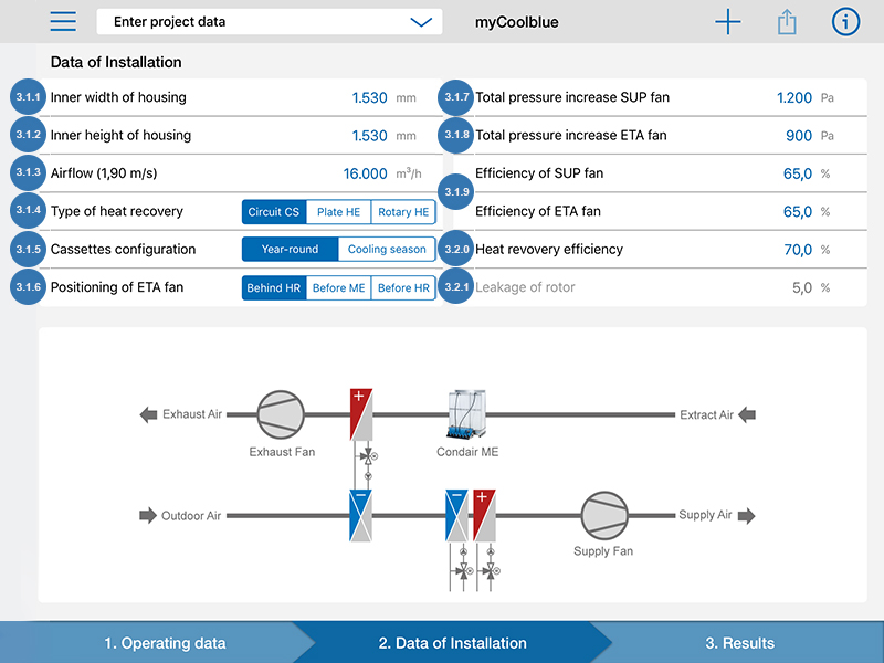
Fig. 3 Data of Installation
3 „Data of Installation“
3.1.1 „Inner width of housing“
The evaporative cooler will normally be integrated into the exhaust device or exhaust system inside of a housing. A larger cross-section yields a lower airflow velocity, which causes a lower air-side pressure drop and thus has a positive effect on the energy contribution. Enter the usable internal width of the exhaust chamber or housing here (see fig. 3).
3.1.2 „Inner height of housing“
Enter the usable internal height of the exhaust chamber or housing here (see fig. 3).
3.1.3 „Airflow“
System nominal flow rate in m³/h. The simulation assumes a constant flow rate with a 1:1 ratio of supply to exhaust air (see fig. 3).
3.1.4 „Type of heat recovery“
Select your intended heat recovery technology here.
Ventilation systems normally use one of three technologies.
CCS: Circuit connected systems with separate heat exchangers which enable you to position the supply and exhaust air systems apart from one another.
PHE: Plate heat exchanger systems require no auxiliary energy and are installed directly between the supply and exhaust air streams. They separate the supply and exhaust air almost entirely using thin plates. They can only be used with connected supply and exhaust air feeds.
RHE: Rotary heat exchangers are also used with connected supply and exhaust air feeds. Depending on the design of the storage mass, moisture may also be transferable. Rotors with moisture transfer capabilities (enthalpy and sorption rotors) are not suitable for use in indirect evaporative cooling. Only condensation rotors can be used. Rotary heat exchangers are often fitted with sliding seals, which can lead to significant leakage from the supply to the exhaust air side. Overflowing humidified exhaust air decreases the savings potential of evaporative cooling, and also increases the amount of energy required to dehumidify the exhaust air
(see fig. 3).
3.1.5 „Cassettes configuration“
You can select whether the humidifier cassettes will remain in the system all year round, or whether they will only be used during the cooler seasons.
As a ventilation component, an evaporative cooler creates a pressure differential in the exhaust air which must be overcome by the fan. This pressure loss normally increases the amount of electrical power required for the extractor fan throughout the entire operational period. The Condair ME evaporative cooler’s cassettes are easy to remove. During the months when external temperatures are lower and evaporative cooling is not required, the cassettes can be removed from the support frame and therefore entirely from the air stream. This decreases the pressure loss to a negligible level, so the extractor fan will require less electricity during this time. This can help you make your evaporative cooling system even more efficient
(see fig. 3).
3.1.6 „Positioning of ETA fan“
The extractor fan can be fitted in one of three different positions in the exhaust device.
Fans warm the air as they apply energy to it. As a rule of thumb, this increase in temperature normally equates to around 1 Kelvin per 1,000 Pa of pressure increase. For example, if the fan is positioned in front of the heat recovery device in the direction of airflow, the 5K drop in temperature created by the evaporative cooler will decrease by some 20% as the extractor fan generates a 1,000 Pa pressure increase. If the extractor fan is, on the other hand, positioned after the heat recovery device in the direction of airflow, the full cooling capacity of the evaporative cooling system will be available.
A third option is if the extractor fan is positioned before the evaporative cooler. The air stream still warms as normal, but in this case, the subsequent evaporative cooler cools it back down to close to wet-bulb temperature. As the temperature before the evaporative cooler is higher than the exhaust air temperature, the exit temperature will also be slightly higher. As you can see, the positioning of the extractor fan represents an opportunity to optimize the evaporative cooler’s energy share
(see fig. 3).
3.1.7 „Total pressure increase SUP fan“
The supply air fan causes an increase in supply air temperature in the same way. The supply air temperature must therefore be lower by the given amount before it reaches the fan. The larger the overall pressure increase caused by the fan, the more cooling capacity will be required to balance out this temperature difference (see fig. 3).
3.1.8 „Total pressure increase ETA fan“
The exhaust air fan also causes an increase in the exhaust air temperature. The results of this are described in more detail in section 3.1.6, “Exhaust air fan position” (see fig. 3).
3.1.9 „Efficiency of SUP/ETA air fan“
The degree of temperature increase in the air stream caused by the fan depends upon its efficiency. The more efficient it is, the lower the temperature increase (see fig. 3).
3.2.0 „Heat recovery efficiency“
The general efficiency of the intended heat recovery device is entered here. The more efficient it is, the more cooling energy can be applied to the supply air via the heat recovery device (see fig. 3).
3.2.1 „Leakage of rotor“
There will normally be a leak between the two air streams in rotary heat exchangers due to their design. Here, you enter the volume of air leakage as a % of the nominal flow rate.
The volume of leakage predominately depends on the pressure difference between the supply and exhaust sides. The positioning of the fans influences both the volume of leakage and the direction of the overflow. The pressure is normally greater on the exhaust air side, which causes the overflow to run from the exhaust to the supply side. Careful positioning of the components can reduce leakage to a minimum and so reduce the increase in supply air humidity caused by overflowing humidified exhaust air
(see fig. 3).
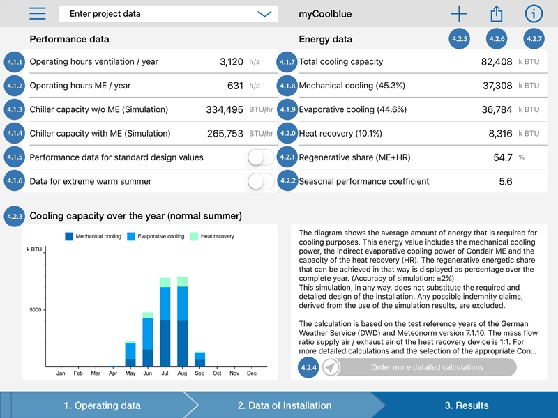
4 Results
The simulation of the ventilation process is based on hourly averages over the course of an observation period. This data is divided into “normal summer” and “extremely warm summer”. Normal summer corresponds with an average summer period. If you select the data for an extremely warm summer, extreme weather conditions occurring within the observation period will also be taken into account (see fig. 4).
4.1.1 „Operating hours ventilation / year“
The annual number of operational hours for the ventilation system is calculated based on the figure provided for the number of days per week the system will be utilized (see fig. 4).
4.1.2 „Operating hours ME / year“
The annual number of operational hours for the evaporative cooler are totaled up and displayed here. If it would be necessary to cool the air during the utilization period, the program will also test whether the evaporative cooling system could be used to pre-cool the external air. If this condition is also fulfilled, the evaporative cooler will be considered active (see fig. 4).
4.1.3 „Chiller capacity w/o ME (Simulation)
Required cooling capacity of the chiller, based on the meteorological data for the selected location and without taking evaporative cooling into account.
When you tap the Cooling capacity for default outdoor conditions button, the app displays the required cooling capacity of the chiller for the selected location at the static design point, without taking evaporative cooling into account
(see fig. 4).
4.1.4 „Chiller capacity with ME (Simulation)“
Required cooling capacity of the chiller, based on the meteorological data for the selected location and taking evaporative cooling into account.
When you tap the Cooling capacity for default outdoor conditions button, the app displays the required cooling capacity of the chiller for the selected location at the static design point, taking evaporative cooling into account (see fig. 4).
4.1.5 „Performance data for standard design values“
To calculate cooling capacity, meteorological data for the selected location are used by default. Use this button to display the cooling capacity for default outdoor conditions.
Note: The results for the required cooling capacity of the chiller under default design conditions may diverge from cooling capacity results based on actual meteorological data (normal or extremely hot summer). The cooling capacity data from the simulation take the normal average values or average extreme values into account, and are not absolute peak values.
When Cooling capacity for default outdoor conditions is selected, no simulation is possible. Instead, the cooling energy diagram and the simulation results for the energy data are displayed in a faded color scheme. The radio button for “Cooling capacity for extremely hot summer” is deactivated in this mode, as are the “Preview” and “Print results” options.
4.1.6 „Data for extreme warm summer“
Meteorological data for normal weather conditions is taken into account as standard. Tap this button to display the simulation results for extremely warm summers (see fig. 4).
Energy data
4.1.7 „Total cooling capacity“
The total annual amount of cooling energy required for the ventilation system to condition the air is displayed here (see fig. 4).
4.1.8 „Mechanical cooling capacity“
Share of the energy which must be produced mechanically if using indirect evaporative cooling, for example via a cold water generator. The percentage of the total cooling energy is displayed in parentheses (see fig. 4).
4.1.9 „Evaporative Cooling“
Share of the cooling energy that can be achieved by using an indirect adiabatic evaporative cooler. The percentage of the total cooling energy is displayed in parentheses (see fig. 4).
4.2.0 „Heat recovery“
Share of the cooling energy which can be achieved by using a heat recovery system. The percentage of the total cooling energy is displayed in parentheses. Cold recovery using a heat recovery system is only possible if the exhaust air temperature is lower than the external air temperature. In some cases, depending on the selected location and the respective operating data for the system, this share may be very small or not available at all (see fig. 4).
4.2.1 „Regenerative share (ME+HR)“
Under certain conditions, the combination of an evaporative cooler and a heat recovery device can be considered an alternative regenerative energy source.
The basic requirement here is that the heat recovery system recovers at least 70% of the heat and the auxiliary energy has a power factor of at least 10 (see fig. 4).
4.2.2 „Seasonal performance coefficient“
The seasonal performance factor indicates the relationship between the amount of thermal cooling energy achievable and the energy consumption necessary to generate it over the course of a year. For mechanical coolers, this is normally between 3 and 5. The higher the value, the more efficiently the thermal cooling energy is generated (see fig. 4).
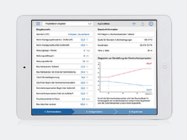
4.2.3 „Bar Chart“
Simulation results are displayed as a bar chart with one bar per month. The data set used, either normal summer or extreme summer, is also displayed in parentheses. The total height of each month’s bar represents the total amount of cooling energy required, and is further divided into mechanical cooling (dark blue), evaporative cooling (light blue) and cooling using only the heat recovery unit (green). In the months where there is no bar, no cooling is required (see fig. 4).
4.2.4 „Order more detailed calculations“
Do you need us to design a Condair ME evaporative cooler for your project? Use this button to send the data you have entered through to us, and we will design a Condair ME evaporative cooler to meet your specific needs. We will assume that you would also like a consultation, and will be in contact shortly.
(see Fig. ).
4.2.5 „+“
New simulation. Selecting a new simulation discards the data you have entered and replaces it with the default values, as when you first launch the program (see fig.).
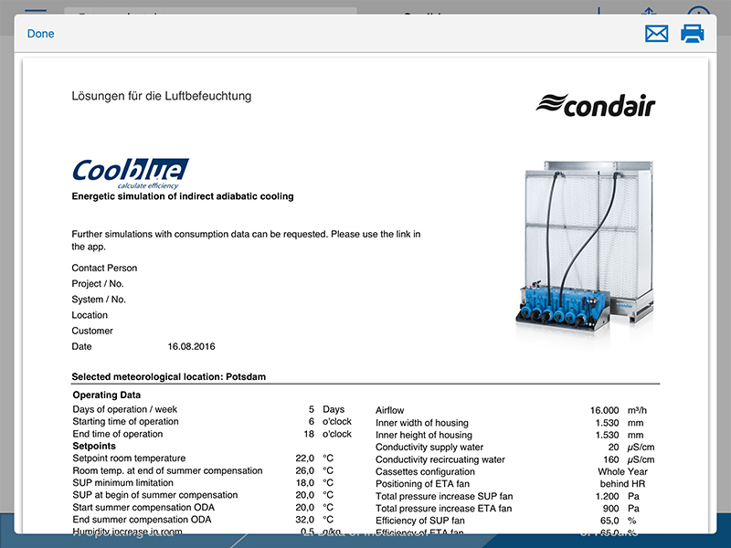
4.2.6 „Send“
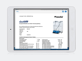
This button generates and displays a preview of the simulation results in PDF format.
This datasheet can be printed via the printer symbol.
You can also send the results via email by tapping the envelope symbol.
The email recipient is set to mycoolblue@condair.com by default. This can be overwritten before sending.
If you send the simulation to mycoolblue@condair.com, we will assume that you require further simulations and advice to plan your project.
(see fig. 4.2.6).
4.2.7 „i“
Use this button to access the Help page (see fig. 4).
Meteonorm is a global meteorological database for engineers, planners and education.
A product of the Meteotest Association, 3012 Bern, Switzerland.
Exclusion of liability:
Simulation is not a substitute for system planning. Our calculations have been developed and prepared with great care, and are based in the best knowledge and belief of Meteonorm. Liability claims and compensation for damages that result from the use of simulation results, or through the use of incorrect or incomplete information, are categorically excluded.
.


